for this problem, I decided to write some code to run the many linear programs for the different facilities. converting it from the written out equations to a linear program was pretty straightforward, just converting a to a sign flipped , and equality into two constraints.
linprog(
    [0, 0, -1 * c[i], -1 * d[i]],
    [
        # -- efficiency within 100%
        # E = (c_i y_1 + d_i y_1) / (a_i x_1 + b_i x_2)
        # E <= 1
        # c_i y_1 + d_i y_1 <= a_i x_1 + b_i x_2
        # -a_i x_1 -b_i x_2 + c_i y_1 + d_i y_1 <= 0
        [-1 * a[k], -1 * b[k], 1 * c[k], 1 * d[k]]
        for k in range(n)
    ] + [
        # -- fixed denominator
        # a_i x_1 + b_i x_2 = 1
        [ 1 * a[i],  1 * b[i], 0, 0],
        [-1 * a[i], -1 * b[i], 0, 0],

        # -- non-negative prices
        # x_1, x_2, y_1, y_2 >= 0
        [-1,  0,  0,  0],
        [ 0, -1,  0,  0],
        [ 0,  0, -1,  0],
        [ 0,  0,  0, -1],
    ],
    [0 for _ in range(n)] + [1, -1, 0, 0, 0, 0],
    bounds=[(None, None), (None, None), (None, None), (None, None)],
)
this runs for the th facility. to figure out how many are relatively optimal, I calculated and checked if its equal to , in which case it’s optimal.
r = c[i] * res[2] + d[i] * res[3]

if r == 1:
    opt += 1
total += 1
since the problem is asking for different variations of the and , I put this into a loop which keeps randomizing those parameters with different numbers of facilities.
n = randint(4, 10)

a = [randint(1, 100) for _ in range(n)]
b = [randint(1, 100) for _ in range(n)]
c = [randint(1, 100) for _ in range(n)]
d = [randint(1, 100) for _ in range(n)]
after running it for a bit, the ratio of seemed to approach .
the second question was what would happen if facilities with more than two inputs/outputs were considered. for this, I moved the script from having separate /// lists and instead having one list with all the parameters. calling it (creatively), this list is indexed like to get the th parameter (first half are input params, second half are output params), and to get the th parameter for the th facility.
n = randint(4, 10)
e = [[randint(1, 100) for _ in range(n)] for _ in range(m * 2)]
I updated the linear program optimization part accordingly.
linprog(
    [0 for _ in range(m)] + [-1 * e[j + m][i] for j in range(m)],
    [
        # -- efficiency within 100%
        # E = (c_i y_1 + d_i y_1) / (a_i x_1 + b_i x_2)
        # E <= 1
        # c_i y_1 + d_i y_1 <= a_i x_1 + b_i x_2
        # -a_i x_1 -b_i x_2 + c_i y_1 + d_i y_1 <= 0
        [-1 * e[j][k] for j in range(m)] + [1 * e[j + m][k] for j in range(m)]
        for k in range(n)
    ] + [
        # -- fixed denominator
        # a_i x_1 + b_i x_2 = 1
        [ 1 * e[j][i] for j in range(m)] + [0 for _ in range(m)],
        [-1 * e[j][i] for j in range(m)] + [0 for _ in range(m)],
    ] + [
        # -- non-negative prices
        # x_1, x_2, y_1, y_2 >= 0
        [0] * j + [-1] + [0] * (m * 2 - j - 1)
        for j in range(m * 2)
    ],
    [0 for _ in range(n)] + [1, -1] + [0] * (m * 2),
    bounds=[(None, None)] * (m * 2),
)
similarly, becomes a sum over the output parameters and coordinating values.
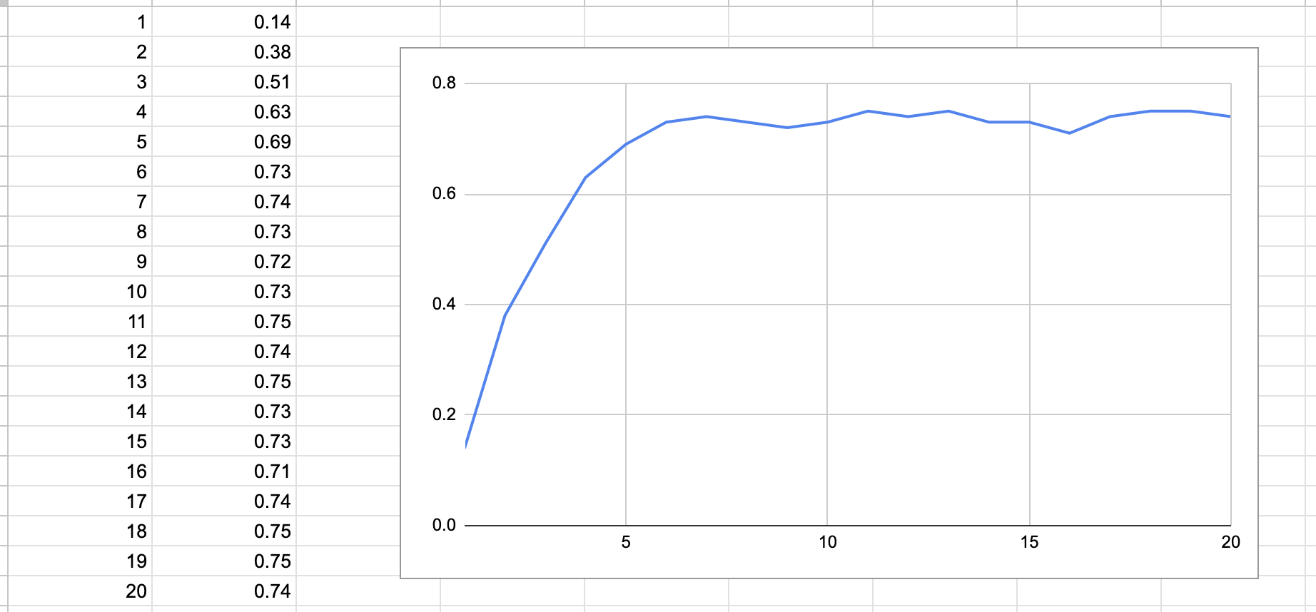
r = sum([e[j + m][i] * res[j + m] for j in range(m)])in order to test out the different parameter counts, I looped over a range of values, which I used to mean the separate count of input/output parameters. putting the ratios I found in a spreadsheet gives this graph of for each param count.
both scripts are in this github repo: https://github.com/ayukmr/dea. inside src/dea, four.py is for 2 params (4 in total) and dynamic.py is for any params.